TAXES (The data that goes with these instructions is in the excel spreadsheet I attached). This problem is an example of a task that might be given to you "in the real world." (Although in the "real...

TAXES (The data that goes with these instructions is in the excel spreadsheet I attached).

This problem is an example of a task that might be given to you "in the real world." (Although in the "real world," you should not expect your boss or client to give you guidance such as "screenshots" or give you hints to help you tackle the problem.) Multiple ways to tackle a problem may be possible, but some methods are much more tedious and/or much less flexible.

HINT: Do NOT use nested IF's (IF functions within IF functions) or the IFS function for the tasks assigned in this problem!

Based on the textbook reading and myNotes file, you should learn: 1) how to determine which functions to use; 2) how to properly create the referencetable_arrays
necessary to use the lookup & referencefunctions; and 3) the correct function arguments to make the function return the desired results.

Note: The information in this Case Problem does not reflect any actual tax rates, tax rate calculation methodologies, or IRS policies, and should not be constituted as tax advice!

The Arlington Group is a "think tank" in Washington, D. C. that provides research data to lobbyists and members of the federal government. As a tax analyst for the Arlington Group, your job is to report how tax policies affect federal, state, and local revenues. A lobbyist asks you to study how alternate flat tax rate proposals could affect the total taxes owed and residual amount of taxes owed on April 15, based on a list of sample individual tax return information. A flat tax rate is a rate applied to the total income earned. For example, a flat tax rate of 10% on $20,000 in income is $2,000. (The current graduated system applies different percentages to ranges of income for each taxpayer. For example, a graduated tax on a $20,000 income might be as follows: 0% of the first $5,000, 10% of the amounts between $5,001 and $10,000, and 15% of the amounts over $10,000.)

A data file is provided that includes schedules for the proposed tax rates, penalties, and state allowances. To complete this study, your task is to analyze the total taxes owed based on two new flat rate tax alternatives. In addition, you will compare the residual amount owed and penalties applied to that residual amount for each alternate. The residual Unpaid Tax owed on April 15 is calculated as follows: tax owed – (withholding taxes paid + estimated taxes paid).

Depending on the amount owed, penalties might be applied to the residual amount owed. Complete the following: (Show all dollar values & percentages to 0 decimal places.)

1.Open the data filetaxes.txtand put the data from the file in a worksheet namedTaxes. (Please remember to include aDocumentationsheet that includes a hyperlink to yourTaxesworksheet.)
Note: Hyperlinks to text files often open directly within web browsers rather than prompting you to download the file. You may copy the data from the web browser, paste it into Excel and then use theText to Columnsfeature (Alt, a, e) to parse the data into separate columns...(Youwill need to pick the correct delimiter to correctly parse the data into separate columns.)

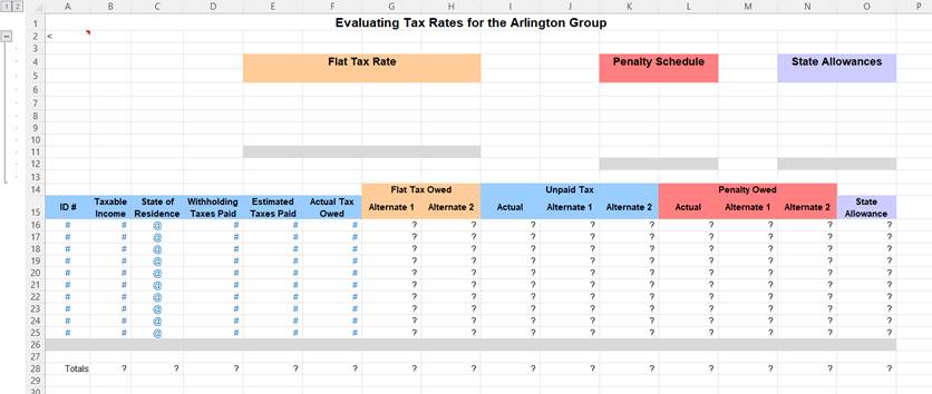
2.Format your worksheet like the image shown. Your spreadsheet should use the same rows/columns and cell placement as shown in the image. Do NOT insert columns or rows, or otherwise rearrange the design of the spreadsheet. Since the spreadsheet should be able to accommodate 1,000 tax ID #'s as easily as 10, make sure the column headings and ID #'s can still be seen, even when scrolling. Format the dollar values such that they align on the left of the column.The dollar signs should show on only the top value in each list of consecutive dollar values.Also show the dollar sign on dollar values that are Totals.Decimal places should line up for all values. Show 0 decimal places for all dollar values.

3.All four digits of Tax ID# should be shown, even if the Tax ID# begins with a 0.

4.Make it so theID#corresponding with thehighestActual Tax Owedis automatically formatted with a bold green font color, and theID#corresponding with thelowestActual Tax Owedis automatically formatted with a bold red font. This formatting should be flexible, so that if any of the Incomes and/or Actual Taxes Owed change, the formatting will automatically adjust to indicate the correct highest and lowest values.

5.Use the information below to construct aFlat Tax Ratetable, which will be used to calculate Flat Taxes owed for various incomes.Show both the min and max values in the table you create.(You may want to refer to my “clear_tables” worksheet in my Notes.)
TIP: It is important that you properly construct your table so that your lookup functions will work!Refer to the Rules I have provided (in my Chapter 5 Notes file) for constructing lookup tables.
For Flat Tax Alternative 1, the following tax rates are applied:
22% tax on incomes of $122,000 or more’
15% tax on incomes of at least $72,000 but less than $122,000;
10% tax on incomes of at least $32,000 but less than $72,000;
3% tax on incomes of at least $15,000 but less than $32,000;
no tax on incomes below $15,000.
For Flat Tax Alternative 2, the following tax rates are applied:
20% tax on incomes of $122,000 or more’
11 tax on incomes of at least $72,000 but less than $122,000;
7% tax on incomes of at least $32,000 but less than $72,000;
5% tax on incomes of at least $15,000 but less than $32,000;
no tax on incomes below $15,000.

6.Ensure that theFlat Tax Ratetable is clear so that anyone viewing the spreadsheet can easily determine the flat tax % rates that are used for each range of income.(Also, a user should be able to edit the values in the table at any time and the table should remain clear and accurate.)
Note: Income is rounded to the nearest dollar, so there is no need to show cents.
TIP: The Flat Tax Rate table shown in the screenshot makes use of an additionalcolumn to display the upperboundaries of the ranges.(The tables shows both the Min & Max values.If needed, you may refer back to my “clear_tables” worksheet in my Notes.)

7.Any dollar values within the data that are 0 should show as a dash. However, in the assumptions (in your reference tables), it makes more sense for 0’s to show rather than dashes.

Hint: To make the accounting format show 0's rather than dashes, you will need to use a custom number format. First apply the accounting format, then change to a custom number format and edit the accounting format code to show a 0 rather than a dash (in the third section of the custom number format code).

Hint2: The Custom number format code contains four sections of code (separated by semi-colons):
1) controls how the number shows when it is positive,
2) controls how the number shows when it is negative,
3) controls how the number shows when it is 0,
4) controls what is shown if text is entered in the cell.

8.In theFlat Tax Owed Alternate 1column,write a formula that uses the Alternate 1 flat tax rate to determine the total dollar value of the tax for the respectiveTaxable Income.
Using theFlat Tax Ratetable, this tax scheme calculates taxes by multiplying the total income by the corresponding rate. Use one of the lookup functions (HLOOKUP or VLOOKUP) as part of your formula for this part. Your formula should beflexible,so that additional rows can be added for additional income brackets.(Although only 2 Flat Tax Alternates currently exist, there could be up to 10 Flat Tax Alternatives.)

9.In theFlat Tax Owed Alternate2column,write a formula that uses the Alternate2 flat tax rate to determine the total dollar value of the tax for the respectiveTaxable Income.
Using theFlat Tax Ratetable, this tax scheme calculates taxes by multiplying the total income by the corresponding rate. Use one of the lookup functions (HLOOKUP or VLOOKUP) as part of your formula for this part. Your formula should beflexible,so that additional rows can be added for additional income brackets.

10.In the first cell under theActual Unpaid Taxescolumn heading, write a formula that calculates the amount of taxes the first taxpayer still owes on April 15. The residual Unpaid Tax owed on April 15 is calculated as follows: tax owed – (withholding taxes paid + estimated taxes paid).
Write the formula so that it can be copied down the column to calculate this amount for each taxpayer (ID #). Also write the formula so that it can be copied across the row to determine the unpaid amount based on the taxes owed for the Alternate 1 and Alternate 2 tax calculations. (Assume the same withholding and estimated taxes paid.) You should be able to enter one formula, then copy it across to the other two columns ofUnpaid Taxes, and copy the same formula(s) down to the other rows within all threeUnpaid Taxcolumns.
Many taxpayers will shownegative numbersfor their Unpaid Tax. If a "Tax Owed" value is negative, then you paid more than you really owe, and therefore the government owes you a refund. Therefore leave the negative numbers to show how much refund is owed.

11.Use the info below to construct a table that will be used as aPenalty Schedule.
Use the range shown in the image provided, where the @ symbols are the headings, and the cells with #'s are for the rest of the data. This table will not showboththe min and max values. Instead, ituses only the breakpoint values required for the lookup function to work properly.

Penalty Schedule Info:

apenalty of 25% is charged on an Unpaid Tax balance of $50,000 or more;
apenalty of 20% is charged on an Unpaid Tax balance of at least $10,000 but less than $50,000;
a penalty of 15% is charged on an Unpaid Tax balance of at least $5,000 but less than $10,000;
apenalty of 10% is charged on an Unpaid Tax balance of at least $1,000 but less than $5,000;
apenalty of 5% is charged on an Unpaid Tax balance of at least $100 but less than $1,000;
and unpaid tax balances of less than $100 owe no penalty.

12.Ensure that thePenalty Scheduletable is clear so that anyone viewing the spreadsheet can easily determine the penalty % charged depending on the amount of unpaid tax owed.(Also, a user should be able to edit the values in the table at any time and the table should remain clear and accurate.) Note: Do notinsert an additional column in order to display boththe lower & upperboundaries of the ranges.The @ symbols at the top of each column of data should be replaced with text labels describing the numbers below.The # symbols should be replaced with numbers.

13.In theActual Penalty Owedcolumn, use thePenalty Scheduleto determines the actual penalty owed.
Please use one of the lookup functions (HLOOKUP or VLOOKUP) aspartof your formula for this part.
Hint:Rather than just looking up the Unpaid Tax in order to find the penalty, use an IF function to determine if the unpaid tax amount is negative, indicating that the IRS owes the taxpayer a refund. If the IRS owes the taxpayer a refund,no penalties apply...therefore make your formula return a value of 0 (but shown as a dash). Copy this formula both down the column to calculate the penalty for the corresponding ID# AND across the row to determine the penalties based on each alternate tax scheme.

14.As part of the flat rate tax, one possible scheme would include a state allowance to balance the high and low cost of living. The amount of the allowance per state is listed as follows: a $600 allowance for OK, a $900 allowance for GA, a $400 for TN, a $400 allowance for SC, a $250 allowance for NC, and an $800 allowance for FL.Construct a table of "State Allowances" to be used for finding the allowance for each taxpayer's ID#. (Use the range shown for the State Allowances in the image provided, where the @ symbols should be replaced with headings describing the data in the column below.The cells with ! should contain either the state abbreviations or the state allowance dollar values.) Note: Your data currently does not include any employees from NC, but make sure your spreadsheet formulas can accommodate employees from this state as well.

15.In theState Allowancescolumn, use formulas to determine the state allowance for each taxpayer.
HINT: Use one of the lookup functions (HLOOKUP or VLOOKUP) for your formula for this part. Allowances for additional states may eventually need to be added as well, so ensure your formula ranges accommodate the possibility of future states being added.
HINT 2:If you have extra spaces within the text of your data or assumptions, then your functions may not appear to work.You can perform a Find/Replace to get rid of extra spaces, or else use the TRIM function, which strips trailing spaces.

16.If the "State of Residence" data contains a state not listed in the State Allowances table (e.g. NY), the State Allowance for that ID# should show the wordNone(not#N/A).
HINT: If you are having trouble with this part, first verify that you have createdthe formula to find the State Allowance for all states that exist in the table. Then, to handle the situations when a state does not exist in the State Allowances table, edit your formula and insert one additional function to make the formula return the wordNone(instead of #N/A). Determine which extra function you need to add. (Your formula will have more than one function in it.)

17.Make it so that the only States that can be entered in the "State of Residence" column are states shown in the State Allowances table (in the assumptions section at the top). When a user wants to enter a state in the State of Residence column, he/sheshould be able to use "pull-down arrows" to select from the list of states in the State Allowance table.Your spreadsheet should prevent future entry of invalid data, but it will not affect data that has already been entered.(Your data could already contain some “invalid data” that will remain within your data.)
HINT:Use Data Validation.This is covered in the Validation & Automation Notes (and in Ch10 of the text).

18.Skip a row beneath the last ID# andincludeTotals for numeric data above, as shown in the screenshot.(Ensure that your formulas are flexible and can always easily accommodate additional rows of data.)The Total at the bottom of the State of Residence column should count the number of States. However, do not worry about counting the unique number of states…just count the number of “rows.”

19.Enter the last four digits of your PID in cell Z100.

20.Make it so that a user can quickly expand (show) and collapse (hide) the rows containing the Tables of Assumptions.
HINT: Note the expandable/collapsible “plus/minus” button to the left of the Row 2 row heading.Please make it so that plus/minus “summary row” button is at the top of the collapsible rows.
Insert a comment in row 2 (in the cell with the “

21.Add your name to the Header of the Page Setup, so it will show when the worksheet is printed.

22.Now make a copy of the “Taxes” sheet and name this new sheet "Taxes (INDEX)".On this sheet, re-do your lookup formulas, using INDEX & MATCHanywhere you previously used a lookup function.

GRANITE (The data that goes with this is the excel spreadsheet I attached).

Granite City Books is planning a $2.5 million expansion of its facilities. It needs to evaluate its options for financing the expansion. The company’s bank might not allow it to obtain more long-term debt financing if its debt-to-equity ratio gets too high. Alternatively, common stockholders might be displeased if their ownership rights become diluted by issuing a substantial amount of preferred stock, or even additional common stock if it is not issued on a pro-rata basis. A workbook has been started that contains a basic balance sheet, solvency, and capital structure ratio data. Your task is to create scenarios for each financing alternative and prepare reports that Granite City Books’ bank and management can use to compare the various financing alternatives.
Note the name of the Scenario is entered in cell A4 and centered across the spreadsheet (through column F). The $ should be directly to the left of any dollar values, but make it so that any dollar values of 0 show up as dashes.
HINT:Apply the Currency Format and then change to a custom number format, where the third section of the custom # format code should contain “-“.Any 0% values should also show as dashes.(However, the actual values should only be custom formatted to show as “-“…the actual values should be 0.Otherwise, those cells would be interpreted as text by the pivot table, which will cause problems.(Pivot Tables need to use number values.)

In case you are curious, the negative $27 (thousand) change in Current Liabilities (and matching positive $27 (thousand) in Retained Earnings) is given to you. It stays the same in all four scenarios. (Assume that no matter which financing option is chosen, the company plans to pay off $27 (thousand) of its Current Liabilities.)

Complete the following:

1.Use the data in theGranite.csvfile & save it in a worksheet named "Options."Then create formulas where appropriate to complete the spreadsheet.For the first year listed as 20XX (column B), replace the XX to show current year.For the second year column heading listed as 20XX (column D), replace the XX to show next year.The formulas for the second year are simply the values in the first year column plus the values in the Changes column.(NOTE:You do not yet know the values for the Changes…C8, C11, C13 & C15.The values for those cells will be provided for you in Step 3.But you can go ahead and enter formulas for those values in the final year regardless.)

Use the following to help you construct formulas for the ratios at the bottom:
Debt-to-equity ratio=Total Liabilities / Total stockholders' equity
Long-term-debt to equity ratio=Long-term Liabilities / Total stockholders' equity
Debt-to-common-equity ratio=Total Liabilities / Common stock
Long-term-debt to common equity=Long-term Liabilities / Common stock
Common-to-preferred equity=Common stock/ Preferred stock
HINT:When entering formulas for the % Change and the ratios (at the bottom), make use of an error-checking function, so that rather than producing a #DIV/0! error, the formula will instead return a value of 0.

Returning a text value, a #N/A or any other non-number can confuse the Scenario Pivot Table and causes it to produce some incorrect results. Therefore your formula CANNOT include a result such as a dash or "0.00%" (with quotation marks around them) since the insertion of quotation marks turns the number into text and your scenario summary and pivot table won't be able to produce correct results with text.
In many situations (such as in this problem), showing dashes (rather than 0’s) may be more appropriate, since showing a value of 0 might be "misleading".Mathematically, you cannot really have a Common to Preferred Equity ratio of 0 when the divisor is 0, so it is better to show the result as a dash rather than a 0.Therefore format your 0% values so that they show as“ - “ (a dash) rather than as 0%.(Show just a plain “-“ without the % for zero values…not “- %”).
NOTE:Your formulas should still return a 0 as the actual value so the pivot tables will work properly.Pivot Tables did not properly with text values.So your formulas should not result in the text value of “-“.

2.Define Names for the worksheet scenarios' changing cells, as shown in Table 8.5 (below). Use abbreviated names for the cell names--it does not matter what names you use, as long as the names are clear (i.e. your names do not have to be the same as the ones the instructor uses).

There is also a negative $27 (thousand) change in Current Liabilities (and matching positive $27 (thousand) in Retained Earnings) that is given to you. It stays the same in all four scenarios, no matter which financing option is chosen, so there’s no need to add it as a changing cell.
In addition to naming the cells listed in the table above, also name cell A4, which should contain the Financing Option shown.

3.Create four scenarios in the Options worksheet using the scenario names and changing cell values shown in Table 8.6, below. (Use the column headings below for your four scenario names.) Do NOT create separate sheets for each Scenario. That's the great thing about scenarios. You do not have to create separate worksheets to show results for different sets of assumptions. All of the different sets of assumptions can be saved within the current worksheet—each as a different scenario.
(All $ values shown in thousands of dollars)

Note: When creating your scenarios, be sure to include the name of your scenario somewhere within the worksheet and include that cell as one of the changing cells. This way, a user can easily tell which scenario is currently being used/shown. For example, the name of the Scenario being displayed in the Options worksheet is included in cell A4 (shown in the screenshot at the bottom), and this value changes to reflect the current scenario being displayed. (Place this scenario name in cell A4 of the Options worksheet, and have it centered across through cell F4.)
Note2: When specifying the changing cells for your various scenarios, use the same changing cells--specified in the same order--for all of your scenarios. Neglecting to do so can cause confusion when you try to create a Scenario Summary PivotTable.
Include a Comment (the new threaded comments, not the old comments with the red triangle) in cell B4 to alert other users to the existence of the Scenarios in the worksheet. (Press Alt, r, c to quickly insert a comment.)Include instructions indicating how to switch between the different sets of assumptions. (Press Alt, a, w, s to access the Scenario Manager.).
NOTE:Older versions of Excel (prior to Excel 365) do not have threaded comments.If it is too much trouble to upgrade your version of Excel or to find a computer that has a more recent version of Excel, you may insert the older style comment (with the red triangle).(For more info, review:The difference between threaded comments and notes - Office Support (microsoft.com))

Normally, I like to customize the Quick Access Toolbar (QAT) to include a button that allows quickly switching between the different scenarios created. (When customizing the QAT, if you clickMore Commands...you will find theScenariopull-down menu underAll Commands.)HOWEVER, there appears to be a bug in the QAT Scenario “quick-switcher”.When switching from the first scenario to any other scenario, a message appears asking if you want to “Redefine your scenario…”Normally this message occurs when you switch from the current scenario back to the same scenario (allowing you to quickly “edit” your scenario values on the fly).But this message is occurring any time you switch away from the current scenario, which can be extremely confusing to users.

(FYI, any QAT customization occurs only on the PC you are using...it does not get saved with the file.)

4.Based on the information in Table 8.7, define appropriate names for the worksheet’s result cells.It does not matter what names you use, as long as the names are clear. (i.e. your names do not have to be exactly the same as shown in the Table).

5.Create a professional-lookingScenario Summaryreport that shows all the results cells listed in Table 8.7. SAVE YOUR FILE BEFORE ATTEMPTING TO RUN THE SCENARIO SUMMARY!Make it so that you can quickly and easily hide or show the row containing the Scenario Name changing cell, and the column containing the Current Values.
When you create the Scenario Summary, it’ll look like the screenshot below. (Your numbers formats should be the same as in the Options worksheet.) Some edits I made were to make the columns thinner; wrap text for the column headings; collapse the row (containing info about the scenario); hide the row containing the names of the Scenario Displayed (since this is redundant info); and hide the column with the "Current Values" (since this is redundant info).

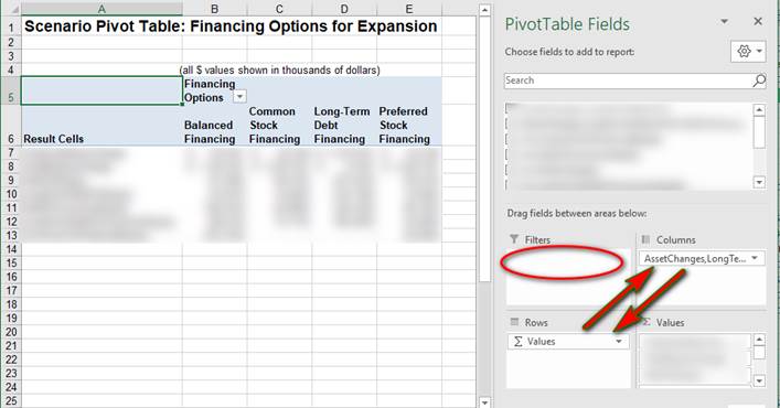
6.Create a professional-lookingScenario PivotTablethat shows all the result cells listed in Table 8.7. (From the Scenario Summary window, just click “Scenario PivotTable report”.

Below is the initial Scenario Pivot Table which is created. (But do not leave your Pivot Table like this.)

Below is an example of the same Pivot Table after fields have been rearranged and formatted.(It takes up less space, and is easier to read.)
To make yours look like the one below, swap the Columns and Rows.

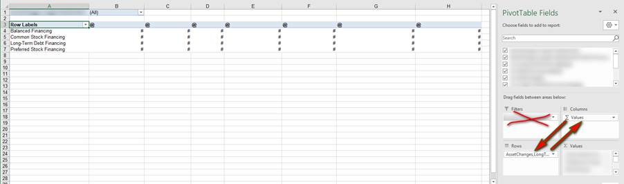
After creating your Scenario Pivot Table, insert two rows at the top of the sheet to make room for the title and a blank row below it. You should not put the title in the cell two rows up from the blue headings, since Row 3 is reserved for when the Report Filter is enabled. This particular pivot table does not need a Report Filter, so that Report Filter area of the Field List can be cleared, and Row 3 will be blank. To remove the report Filter drag the item from the Filter area.Also, manually edit cell B5 toread "Financing Options"...which is much more clear than "Column names."

7.Follow the homework guidelines for properly submitting your homework. (Also, arrange your sheets in the order of the steps.Put Documentation first, then Options, then Scenario Summary, then Scenario PivotTable.)